2層のニューラルネットワークをスクラッチから実装
やりたいことは2階層のニューラルネットワークを実装して、猫なのか、猫じゃないなのかを判断するモデルを作ることです。CNN(畳み込みネットワーク)は使わず、スクラッチからNumpyでForward PropagationとBack propagationを実装します。
209枚の画像訓練データと50枚の画像テストデータを使います。
訓練データtrain_catvnoncat.h5とテストデータ test_catvnoncat.h5両方とも HDF5フォーマットです。
とりあえず訓練データを読み込んで中身を確認します。
import numpy as np
import h5py
train_dataset = h5py.File('./images/train_catvnoncat.h5', "r")
print(list(train_dataset.keys()))
結果
['list_classes', 'train_set_x', 'train_set_y']
訓練データの画像セットとラベルをそれぞれ抽出します。訓練用の画像は209枚があって、どれも3つの色チャンネルで、 横 x 縦 64 x 64の画像です。
train_x_orig = np.array(train_dataset["train_set_x"]) # 訓練データ画像セット自体
train_y = np.array(train_dataset["train_set_y"]) # 訓練データ画像セットのラベル
train_y = train_y.reshape(train_y.shape[0], -1).T

print(train_x_orig.shape)
print(train_y.shape)
結果:
(209, 64, 64, 3)
(1, 209)
訓練データと同様にテストデータを準備します。テストの画像データは50枚があって、どれも3つの色チャンネルで、 横 x 縦は 64 x 64の画像です。
test_dataset = h5py.File('./images/test_catvnoncat.h5', "r")
test_x_orig = np.array(test_dataset["test_set_x"]) # テストデータ画像セット自体
test_y = np.array(test_dataset["test_set_y"]) # テストデータ画像セットのラベル

test_y = test_y.reshape(test_y.shape[0], -1).T

print("test_x.shape: ", test_x_orig.shape)
print("test_y.shape: ", test_y.shape)
テストデータの中でどんなラベルあるかを見てみると、non-catと cat二種類データは入っています。
list(train_dataset['list_classes'])
結果:
[b'non-cat', b'cat']
実際画像を表示して、ラベルは1の場合猫であることがわかります。
import matplotlib.pyplot as plt
%matplotlib inline
index = 2
plt.imshow(train_x_orig[index])
plt.show()
print("猫: ", train_y[0, 2])
結果:
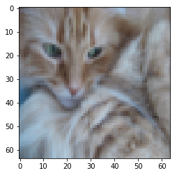 猫: 1
猫: 1
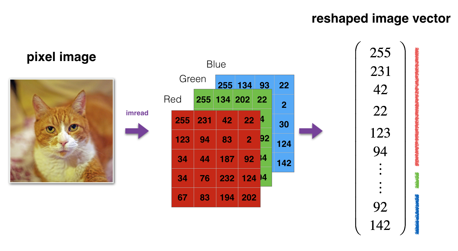
画像をニューラルネットワークに入れる前にまず一個のベクトルにしておきたいので、下の変形を行って、縦(一枚の画像)は 12288(64 * 64 * 3)のNumpy配列に直します。
m_train = train_x_orig.shape[0]

m_test = test_x_orig.shape[0]

train_x_flatten = train_x_orig.reshape(m_train,  -1).T

test_x_flatten = test_x_orig.reshape(m_test, -1).T

print(train_x_flatten.shape)

print(test_x_flatten.shape)
結果:
(12288, 209)
(12288, 50)
画像のピクセルの値は [0,255] の間なので、ニューラルネットワークに入れる前にピクセルの値を正規化しておきます。訓練データとテストデータ両方とも正規化を行います。
train_x = train_x_flatten / 255.
test_x = test_x_flatten / 255.

print ("train_x's shape: " + str(train_x.shape))
print ("test_x's shape: " + str(test_x.shape))
結果:
train_x's shape: (12288, 209)
test_x's shape: (12288, 50)
これで訓練データを把握したので、2層のニューラルネットワークを作ってみます。このネットワークの構造は下の図で表現しています。
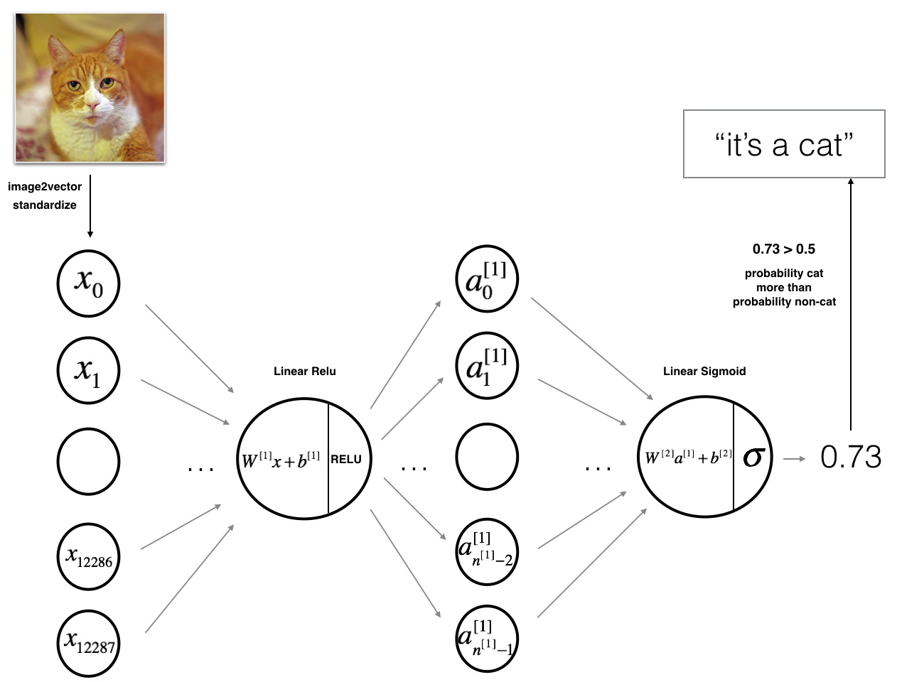 画像の入力はレイヤー0とみなしてよくて、 $W^{[1]}$ は レイヤー1の出力のための重みで、ランダムに初期化する必要があります。$b^{[1]}$はレイヤー1のbiasで、特にランダムに初期化する必要はなく、全部ゼロにしておきます。
def initialize_parameters(n_x, n_h, n_y):
    """
    引数:
    n_x -- 入力層(input layer)のサイズ、上の例では n_x = 12288
    n_h -- 隠れ層(hidden layer)のサイズ
    n_y -- 出力層(output layer)のサイズ、non-catとcat二種類だったら、n_y=2になる

    戻り値:
    parameters -- Pythonの辞書型オブジェクト:
                    W1 --  1層目の重みで、マトリックスの shapeは  (n_h, n_x)
                    b1 -- バイアス(bias)のベクトル、 shapeは (n_h, 1)
                    W2 -- 2層目の重みで、マトリックスの shapeは (n_y, n_h)
                    b2 -- 2層目のバイアス(bias) ベクトルで、 shapeは (n_y, 1)
    """

    np.random.seed(1) # 毎回同じ結果得られるようにseedを設定しておく

    # 1層目の重みとバイアスを初期化する
    W1 = np.random.randn(n_h, n_x) * 0.01 # 0.01を掛けないと数字は少し大きいため
    b1 = np.zeros(shape=(n_h, 1))

    # 2層目の重みとバイアスを初期化する
    W2 = np.random.randn(n_y, n_h) * 0.01
    b2 = np.zeros(shape=(n_y, 1))

    assert(W1.shape == (n_h, n_x))
    assert(b1.shape == (n_h, 1))
    assert(W2.shape == (n_y, n_h))
    assert(b2.shape == (n_y, 1))

    # 初期化した結果をparameters 辞書型として返す
    parameters = {"W1": W1,
                  "b1": b1,
                  "W2": W2,
                  "b2": b2}

    return parameters
initialize_parameters関数は2層(入力層入っていない)のニューラルネットワークを初期化(W1, b1, W2, b2)しました。L層のニューラルネットワークを初期化する場合は少し複雑です。$n^{[L]}$はL層のノードの数とみなしていいです。
| Shape of W | Shape of b | Activation | Shape of Activation | |
| Layer 1 | $(n^{[1]},12288)$ | $(n^{[1]},1)$ | $Z^{[1]} = W^{[1]} X + b^{[1]} $ | $(n^{[1]},209)$ |
| **Layer 2** | $(n^{[2]}, n^{[1]})$ | $(n^{[2]},1)$ | $Z^{[2]} = W^{[2]} A^{[1]} + b^{[2]}$ | $(n^{[2]}, 209)$ |
| $\vdots$ | $\vdots$ | $\vdots$ | $\vdots$ | $\vdots$ |
| Layer L-1 | $(n^{[L-1]}, n^{[L-2]})$ | $(n^{[L-1]}, 1)$ | $Z^{[L-1]} = W^{[L-1]} A^{[L-2]} + b^{[L-1]}$ | $(n^{[L-1]}, 209)$ |
| Layer L | $(n^{[L]}, n^{[L-1]})$ | $(n^{[L]}, 1)$ | $Z^{[L]} = W^{[L]} A^{[L-1]} + b^{[L]}$ | $(n^{[L]}, 209)$ |
ニューラルネットワークののForward Propagationの線形部分を計算する際に$Z = WX + b$を使っています。
これでニューラルネットワークの初期化を完了したので、Forward Propagationを実装する段階に入ります。3レイヤーのニューラルネットワークの場合、レイヤー0(画像データの入力層)からレイヤー1の出力結果を計算するために下の方法を使います。
$Z^{[l]} = W^{[l]}A^{[l-1]} +b^{[l]}\tag{4}$
$l=1$の時に、 $A^{[0]}$は入力データで、線形部分$W^{[l]}A^{[l-1]}$を計算する際に numpy.dot(W, A)を使うといいです。
def linear_forward(A, W, b):
    """
    Forward Propagationの各レイヤーの線形部分を実装する

    引数:
    A -- Activation関数適応した後前のレイヤーの出力結果(あるいはレイヤー0入力層)、Shapeは
    (前のレイヤーの次元, 入力サンプルの数)
    W -- 重みのマトリックス: Shapeは(現在レイヤーの次元, 前のレイヤーの次元)
    b -- バイアスベクトル, Shapeは(現在レイヤーの次元, 1)

    戻り値:
    Z -- WA+bの結果, Zに対して、Activation関数を適応する
    cache -- Pythonの辞書、 "A", "W" and "b" は入っている。 Back Propagationを計算する際に使われる。
    """
    Z = np.dot(W, A) + b

    assert(Z.shape == (W.shape[0], A.shape[1]))
    cache = (A, W, b)

    return Z, cache
そして$Z$に対してActivation関数を適応して、$\sigma(Z) = \sigma(W A + b)$になります。よく使われるActivation関数の二つは Sigmoidと ReLU関数です。
Sigmoidの場合: $\sigma(Z) = \sigma(W A + b) = \frac{1}{ 1 + e^{-(W A + b)}}$
ReLUの場合:$\sigma(Z) = \sigma(W A + b) = ReLU(Z) = max(0, Z)$
def sigmoid(Z):
    """
    Sigmoid というActivation関数を実装

    引数:
    Z -- ShapeはWAで決まる

    戻り値:
    A -- sigmoid(Z), Sigmoid関数を適応した出力、Shapeは Zと同じ
    cache -- Zを返す、Back Propagationに使われる
    """

    A = 1/(1 +np.exp(-Z))
    cache = Z

    return A, cache


def relu(Z):
    """
    ReLU というActivation関数を実装

    引数:
    Z -- ShapeはWAで決まる
    Returns:
    A -- relu(z), ReLU関数を適応した出力、Shapeは Zと同じ
    cache -- Zを返す、Back Propagationに使われる
    """

    A = np.maximum(0,Z)

    assert(A.shape == Z.shape)

    cache = Z
    return A, cache

def linear_activation_forward(A_prev, W, b, activation):
    """
    Forward Propagation の  LINEAR->ACTIVATION 部分を実装する関数

    引数:
    A_prev -- 前のレイヤーの結果(あるいは画像入力データのレイヤー0)、Shapeは (前のレイヤーの次元, 入力サンプルの数)
    W -- 重みのマトリックス: Shapeは(現在レイヤーの次元, 前のレイヤーの次元)
    b -- バイアスベクトル, Shapeは(現在レイヤーの次元, 1)
    activation -- 現在のレイヤーに使うActivation関数,  "sigmoid" あるいは "relu"文字列

    Returns:
    A -- Zに対して、Activation関数を適応した後の出力
    cache -- Python辞書で、 Back Propagationのために "linear_cache" と "activation_cache"を保存する
    """

    if activation == "sigmoid":
        # "A_prev, W, b"をInputして、 "A, activation_cache"をOutputする
        Z, linear_cache = linear_forward(A_prev, W, b) #  A_prev, W, bをそのまま保存しておく
        A, activation_cache = sigmoid(Z) # activation_cacheはZのこと


    elif activation == "relu":
        # "A_prev, W, b"をInputして、"A, activation_cache"をOutputする
        Z, linear_cache = linear_forward(A_prev, W, b) #  A_prev, W, bをそのまま保存しておく
        A, activation_cache = relu(Z) # activation_cacheはZのこと


    assert (A.shape == (W.shape[0], A_prev.shape[1]))
    cache = (linear_cache, activation_cache)

    return A, cache
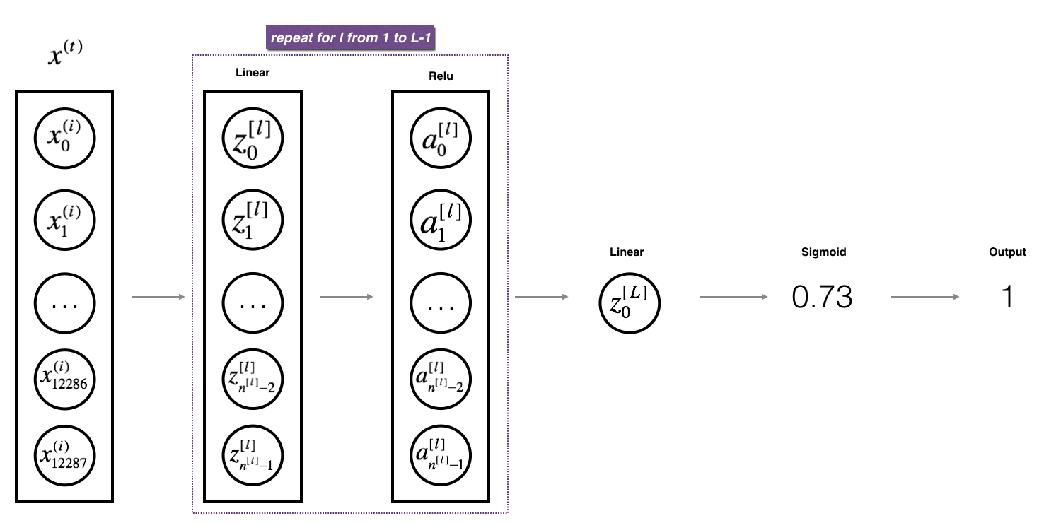
linear_activation_forward関数を実装したことによって、L層のニューラルネットワークを実装するためのかなり便利なパーツが
できました。L層のニューラルネットワークは下の図で表しています。
def L_model_forward(X, parameters):
    """
    Forward Propagationの一連の流れ [LINEAR->RELU]*(L-1)->LINEAR->SIGMOID を実装する

    引数:
    X -- 画像データ, Numpyの配列で、 Shapeは (画像の次元, 画像の数)、例えば上の例だと(12288, 209)
    parameters --  initialize_parameters_deep()関数で初期化したパラメータ、各層の重みWとバイアスbが入っている

    Returns:
    AL -- 最後の層の出力
    caches -- list of caches containing:
                every cache of linear_relu_forward() (there are L-1 of them, indexed from 0 to L-2)
                the cache of linear_sigmoid_forward() (there is one, indexed L-1)
    """

    caches = []
    A = X
    L = len(parameters) // 2                  # number of layers in the neural network

    #  [LINEAR -> RELU]*(L-1) 部分を実装
    for i in range(1, L):
        A_prev = A
        A, cache = linear_activation_forward(A_prev,
                                             parameters['W' + str(i)],
                                             parameters['b' + str(i)],
                                             activation='relu')
        caches.append(cache)


    #  LINEAR -> SIGMOIDの部分を実装する
    AL, cache = linear_activation_forward(A,
                                          parameters['W' + str(L)],
                                          parameters['b' + str(L)],
                                          activation='sigmoid')
    caches.append(cache)

    assert(AL.shape == (1, X.shape[1]))

    return AL, caches
Forward Propagationは後最後の損失関数(Cost Function)で、完了します。モデルを訓練する目標は損失関数をできるだけ小さくしたいです。
クロスエントロピー(cross-entropy)関数を損失関数として使うので、それを実装します。
クロスエントロピー関数は下の形です。
$$ -\frac{1}{m} \sum\limits_{i = 1}^{m} (y^{(i)}\log\left(a^{L}\right) + (1-y^{(i)})\log\left(1- a^{L}\right)) \tag{7} $$
def compute_cost(AL, Y):
    """
    Implement the cost function defined by equation (7).

    Arguments:
    AL -- probability vector corresponding to your label predictions, shape (1, number of examples)
    Y -- ラベルのベクトル例えば、  0 は non-cat, 1 は cat, Shapeは (1, 訓練画像の枚数)

    Returns:
    cost -- クロスエントロピー
    """

    m = Y.shape[1]

    # ALとYで損失関数を実装する。
    cost = (-1.0 / m) * np.sum(np.multiply(Y, np.log(AL)) + np.multiply(1 - Y, np.log(1 - AL)))

    cost = np.asscalar(cost)

    return cost
線形部分の計算で$Z^{[l]} = W^{[l]} A^{[l-1]} + b^{[l]}$
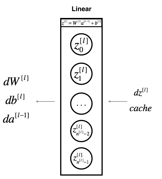
仮に$Z$の微分がわかったとして、 $dZ^{[l]} = \frac{\partial \mathcal{L} }{\partial Z^{[l]}}$. $dZ$を利用して $(dW^{[l]}, db^{[l]} dA^{[l-1]})$を求めたい。
$$ dW^{[l]} = \frac{\partial \mathcal{L} }{\partial W^{[l]}} = \frac{1}{m} dZ^{[l]} A^{[l-1] T} $$
$$ db^{[l]} = \frac{\partial \mathcal{L}}{\partial b^{[l]}} = \frac{1}{m} \sum_{i = 1}^{m} dZ^{[1] [i] } $$
$$ dA^{[l-1]} = \frac{\partial \mathcal{L} }{\partial A^{[l-1]}} = W^{[l] T} dZ^{[l]} $$
def linear_backward(dZ, cache):
    """
    線形部分の逆伝播(Back Propagation)を実装する

    引数:
    dZ -- 現在の層の損失関数の線形部分Zによる変化量
    cache -- forward porpagationのタイミングで現在の層の (A_prev, W, b)を保存したキャッシュ

    戻り値:
    dA_prev -- 前の層(l-1)損失関数のActivation function部分Aによる変化量、shape は A_prevと同じ
    dW -- 現在の層の損失関数の線形部分Wによる変化量、Shapeは Wと同じ
    db -- 現在の層の損失関数の線形部分bによる変化量、Shapeは bと同じ
    """
    A_prev, W, b = cache
    m = A_prev.shape[1]

    dW = 1./m * np.dot(dZ, A_prev.T)
    db = (1./m) *  np.sum(dZ, axis=1, keepdims=True)

    dA_prev = np.dot(W.T, dZ)

    assert (dA_prev.shape == A_prev.shape)
    assert (dW.shape == W.shape)

    return dA_prev, dW, db
Activaton function部分の逆伝播linear_activation_backwardを実装する前にまずsigmoid関数とrelu関数の微分を求める必要があります。ここで重要なのは もし$g(.)$は activation functionであれば、l層のsigmoid_backwardと relu_backwark関数は下のように計算されます。
$$dZ^{[l]} = dA^{[l]} * g’(Z^{[l]})$$
def sigmoid_backward(dA, cache):
    """
    sigmoid関数部分の逆伝播を求める。
    引数:
    dA -- 損失関数のAによる変化量。
    cache -- forward propagationを計算するときにキャッシュとして保存したZ
    戻り値:
    dZ -- 損失関数のZによる変化量。
    """

    Z = cache
    s = 1/(1+np.exp(-Z))
    dZ = dA * s * (1-s)
    assert (dZ.shape == Z.shape)
    return dZ

def relu_backward(dA, cache):
    """
    ReLU部分の逆伝播を実装する

    引数:
    dA -- 損失関数のAによる変化量。
    cache -- forward propagationを計算するときにキャッシュとして保存したZ
    戻り値:
    dZ -- 損失関数のZによる変化量。
    """

    Z = cache
    dZ = np.array(dA, copy=True)

    dZ[Z <= 0] = 0

    assert (dZ.shape == Z.shape)

    return dZ


def linear_activation_backward(dA, cache, activation):
    """
    Activation Function部分 (LINEAR->ACTIVATION ) の逆伝播を実装する

    Arguments:
    dA -- 現在の層の損失関数のAによる変化量。
    cache -- forward propagationを計算するときにキャッシュとして保存した (linear_cache, activation_cache)
    activation -- forward propagationを計算するときに使用したActivation Fucntion,  "sigmoid" と "relu"のどっちか

    戻り値:
    dA_prev -- 前の層(l-1)損失関数のActivation function部分Aによる変化量、shape は A_prevと同じ
    dW -- 現在の層の損失関数の線形部分Wによる変化量、Shapeは Wと同じ
    db -- 現在の層の損失関数の線形部分bによる変化量、Shapeは bと同じ
    """
    linear_cache, activation_cache = cache

    if activation == "relu":
        dZ = relu_backward(dA, activation_cache)

    elif activation == "sigmoid":
        dZ = sigmoid_backward(dA, activation_cache) # dA2と Zを使って、 Zに関する偏微分
        #print("linear_activation_backward,sigmoid, dZ.shape: ", dZ.shape)
    dA_prev, dW, db = linear_backward(dZ, linear_cache) # dZ2はすでにdAから求められている

    return dA_prev, dW, db
$dW$, $db$など求められたので、l層のパラメータの更新は行うことができます。
$$ W^{[l]} = W^{[l]} - \alpha \text{ } dW^{[l]} $$ $$ b^{[l]} = b^{[l]} - \alpha \text{ } db^{[l]} $$
def update_parameters(parameters, grads, learning_rate):
    """
    最急降下法(gradient descent)を使ってパラメータを更新する

    引数:
    parameters -- parameters["W1"], parameters["W2"], parameters["b1"], parameters["b2"]のようなデータ入っている
    grads --  grads['dW1'] grads['db1'], grads['dW2'], grads['db1']のような値は入っている

    Returns:
    parameters -- 更新されたパラメータ
                  parameters["W" + str(l)] = ...
                  parameters["b" + str(l)] = ...
    """

    L = len(parameters) // 2 # number of layers in the neural network

    # forループを使って、パラメータを更新
    for i in range(L):
        parameters["W" + str(i + 1)] = parameters["W" + str(i + 1)] - learning_rate * grads["dW" + str(i + 1)]
        parameters["b" + str(i + 1)] = parameters["b" + str(i + 1)] - learning_rate * grads["db" + str(i + 1)]
    return parameters
2層のニューラルネットのの計算は *LINEAR -> RELU -> LINEAR -> SIGMOID*のような流れになっています。
def initialize_parameters(n_x, n_h, n_y):
    ...
    return parameters
def linear_activation_forward(A_prev, W, b, activation):
    ...
    return A, cache
def compute_cost(AL, Y):
    ...
    return cost
def linear_activation_backward(dA, cache, activation):
    ...
    return dA_prev, dW, db
def update_parameters(parameters, grads, learning_rate):
    ...
    return parameters
実際の実装はtwo_layer_modeにまとめられています。
def two_layer_model(X, Y, layers_dims, learning_rate=0.0075, num_iterations=3000, print_cost=False):
    """
    Implements a two-layer neural network: LINEAR->RELU->LINEAR->SIGMOID.

    Arguments:
    X -- 入力画像データ, Shape (n_x, 画像の枚数) (12288, 209)のようなShape
    Y -- 1は猫、0は猫じゃない。 (1, 209)のようなShape
    layers_dims -- 各層の次元 (n_x, n_h, n_y), (12288, 7, 1)のようなShape
    num_iterations --  loopの回数。例えば2500
    learning_rate -- 勾配降下法に使われる学習率
    print_cost -- trueにすると100回ループしたら一回costをプリントアウト

    Returns:
    parameters --  W1, W2, b1 ,  b2
    """

    np.random.seed(1)
    grads = {}
    costs = []                              # to keep track of the cost
    m = X.shape[1]                           # number of examples
    (n_x, n_h, n_y) = layers_dims

    # ニューラルネットワークのW1, W2, b1, b2を初期化する
    parameters = initialize_parameters(n_x, n_h, n_y)

    W1 = parameters["W1"]
    b1 = parameters["b1"]
    W2 = parameters["W2"]
    b2 = parameters["b2"]


    for i in range(0, num_iterations):
        A1, cache1 = linear_activation_forward(X, W1, b1, 'relu')
        A2, cache2 = linear_activation_forward(A1, W2, b2, 'sigmoid')


        # 損失を計算
        cost = compute_cost(A2, Y)

        dA2 = - (np.divide(Y, A2) - np.divide(1 - Y, 1 - A2)) #  dA2.shape:  (1, 209)


        dA1, dW2, db2 = linear_activation_backward(dA2, cache2, 'sigmoid')
        dA0, dW1, db1 = linear_activation_backward(dA1, cache1, 'relu')

        grads['dW1'] = dW1
        grads['db1'] = db1
        grads['dW2'] = dW2
        grads['db2'] = db2

        # パラメータを更新する
        parameters = update_parameters(parameters, grads, learning_rate)

        W1 = parameters["W1"]
        b1 = parameters["b1"]
        W2 = parameters["W2"]
        b2 = parameters["b2"]

        # Print the cost every 100 training example
        if print_cost and i % 100 == 0:
            print("Cost after iteration {}: {}".format(i, np.squeeze(cost)))
        if print_cost and i % 100 == 0:
            costs.append(cost)


    plt.plot(np.squeeze(costs))
    plt.ylabel('cost')
    plt.xlabel('iterations (per tens)')
    plt.title("Learning rate =" + str(learning_rate))
    plt.show()

    return parameters
n_x = 12288 # num_px * num_px * 3
n_h = 7
n_y = 1
layers_dims = (n_x, n_h, n_y)
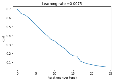
parameters = two_layer_model(train_x, train_y, layers_dims = (n_x, n_h, n_y), num_iterations = 2500, print_cost=True)
結果:
Cost after iteration 0: 0.693049735659989
Cost after iteration 100: 0.6464320953428849
Cost after iteration 200: 0.6325140647912677
Cost after iteration 300: 0.6015024920354665
Cost after iteration 400: 0.5601966311605747
Cost after iteration 500: 0.5158304772764729
Cost after iteration 600: 0.47549013139433266
Cost after iteration 700: 0.4339163151225749
Cost after iteration 800: 0.4007977536203889
Cost after iteration 900: 0.3580705011323798
Cost after iteration 1000: 0.3394281538366412
Cost after iteration 1100: 0.3052753636196265
Cost after iteration 1200: 0.2749137728213017
Cost after iteration 1300: 0.24681768210614838
Cost after iteration 1400: 0.19850735037466102
Cost after iteration 1500: 0.1744831811255665
Cost after iteration 1600: 0.17080762978095967
Cost after iteration 1700: 0.11306524562164735
Cost after iteration 1800: 0.09629426845937154
Cost after iteration 1900: 0.08342617959726858
Cost after iteration 2000: 0.0743907870431908
Cost after iteration 2100: 0.06630748132267929
Cost after iteration 2200: 0.05919329501038168
Cost after iteration 2300: 0.053361403485605544
Cost after iteration 2400: 0.04855478562877018
def predict(X, y, parameters):
    """
    テストデータを使ってニューラルネットのの結果を予測.

    引数:
    X -- 訓練データ
    parameters -- モデルのパラーメータ

    戻り値:
    p -- 予測値
    """

    m = X.shape[1]
    n = len(parameters) // 2 # number of layers in the neural network
    p = np.zeros((1, m),dtype=int)

    # Forward propagation
    probas, caches = L_model_forward(X, parameters)


    # convert probas to 0/1 predictions
    for i in range(0, probas.shape[1]):
        if probas[0,i] > 0.5:
            p[0,i] = 1
        else:
            p[0,i] = 0

    # 結果を出力
    #print ("predictions: " + str(p))
    #print ("true labels: " + str(y))
    print("Accuracy: %s" % str(np.sum(p == y)/float(m)))

    return p
pred_train = predict(train_x, train_y, parameters)
結果:
Accuracy: 1.0
テストデータを予測してみる
pred_test = predict(test_x, test_y, parameters)
結果:
Accuracy: 0.72
https://www.coursera.org/learn/neural-networks-deep-learning