R入門5

We flip the coin 30 times and observe 10 head. We can use R to tell us the probability of getting 10 or fewer heads using the pbinom function.

pbinom(10, size=30, prob=0.5)

0.0493685733526945

The way we determined the probability of getting exactly 10 heads is by using the probability formula for Bernoulli trials. The probability of getting k successes in n trials is equal to:

$$\binom{n}{k}p^k(1-p)^{n-k}$$

rnorm is the R function that simulates random variates having a specified normal distribution. Let’s say there are only 10,000 US women.

set.seed(2)
all.us.women <- rnorm(10000, mean=65, sd=3.5)

# take a random sample of 10 from this population using the sample function 
our.sample <- sample(all.us.women, 10)

print(mean(our.sample))

[1] 66.15138

Note that as we increase the sample size, the sample mean isn’t always closer to the population mean, but is will be closer on average.

population.mean <- mean(all.us.women)

for (sample.size in seq(5, 30, by=5)) {
    
    # create empty vector with 1000 elements
    sample.means <- numeric(length=1000)
    
    for( i in 1:1000) {
        sample.means[i] = mean(sample(all.us.women, sample.size))

    }
    
    distances.from.true.mean <- abs(sample.means - population.mean) ## abs(vector - number)
    
    mean.distances.from.true.mean <- mean(distances.from.true.mean)
    
    print(mean.distances.from.true.mean)
}

[1] 1.222905
[1] 0.9099672
[1] 0.6953492
[1] 0.6083053
[1] 0.5603942
[1] 0.5105878

We are going to take samples of 40 from the population 10,000 times and plot a frequency distribution of the means.

library(ggplot2)
mean.of.our.samples <- numeric(10000)
for (i in 1:10000) {
    a.sample <- sample(all.us.women, 40)
    mean.of.our.samples[i] = mean(a.sample)
}


dat = data.frame("mean.height" =mean.of.our.samples)
ggplot(dat, aes(x=mean.height) ) + 
    geom_histogram(bins=80)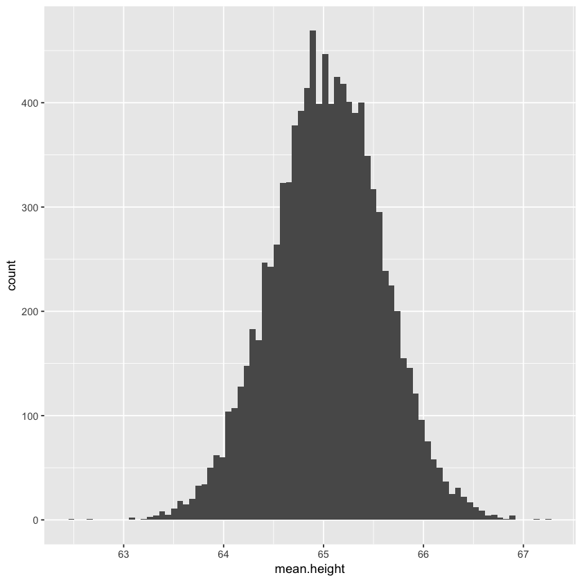

The requency distribution above is called a sample distribution. For a large enough sample size, the sampling distribution of any population will be appromimately normal with a mean equal to the population mean $\mu$ , and a standard deviation of : $$\frac{\sigma}{\sqrt{N}}$$ where N is the sample size and $\sigma$ is the population standard deviation. This is called the central limit theorem

The standard deviation of the sampling distribution is called the standard error and we can use it to quantify our uncertainty about our estimate of the population mean.